
起因
大物实验如果不要报告还是很有趣的,而要写实验报告就很让人崩溃。
霍尔效应这实验不仅数据多,还需要进行很复杂的数据处理及图像绘制。好在老师允许使用Origin,Matlab,Mathematica,LaTeX,…,所以我选用了matplotlib🤣,毕竟有numpy加持的Python再好用不过了
csv读写
当在处理数据的时候,当然还是用Excel比较方便,将数据储存为csv格式就可以很方便地与Python交换数据,但网上对csv模块的介绍质量普遍很低,我这里只使用了DictReader这种方式,把每一行作为一个字典来读取。而csv在保存的过程中必须保证表格是完整的,虽然可以访问空数据,可这样一点也不优雅😢
Matplotlib操作
最重要的就是画图了,由于作图要求是画出折线图和描点,只要分为两次就行。Matplotlib本身支持一些基本LaTeX语法,注意在字符串里写反横杠需要两个来转译。如果使用rcParams里开启usetex就可以使用LaTeX渲染,进而支持更多公式,只不过当然速度极慢。另外,Matplotlib也需要引入新字体才能支持中文渲染。
numpy数据处理
numpy在批量处理数据的时候真是十分方便,这里着重说一下polyfit这个函数,是通过对指定次数的多项式函数去拟合给出的点,一维情况便可以代替手写的最小二乘法。
Examples

 输出:
输出:
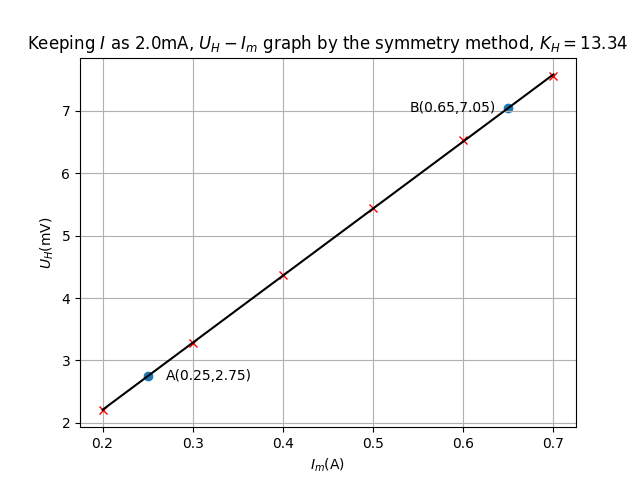
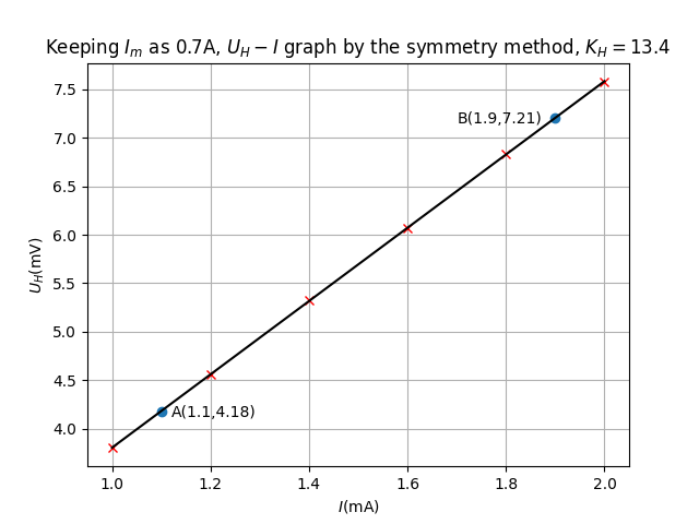
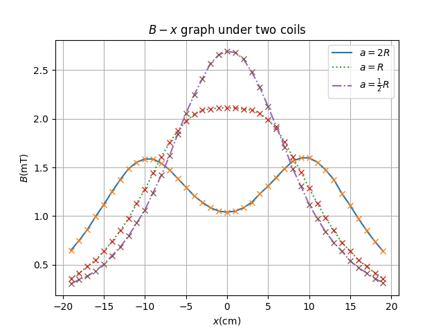
Keep Im UH = [3.8, 4.56, 5.32, 6.07, 6.83, 7.58] B = 2.821kGS KH = 13.399503722084367 Keep I UH = [2.2, 3.28, 4.37, 5.44, 6.53, 7.56] B’ = 8.06kGS KH = 13.335696561503012 Coils one coil = [0.16, 0.18, 0.2, 0.23, 0.26, 0.29, 0.34, 0.38, 0.45, 0.51, 0.59, 0.68, 0.78, 0.89, 1.02, 1.15, 1.26, 1.37, 1.45, 1.46, 1.45, 1.41, 1.33, 1.22, 1.11, 0.97, 0.85, 0.74, 0.64, 0.49, 0.47, 0.41, 0.35, 0.3, 0.26, 0.22, 0.2, 0.17, 0.15] 2R = [0.65, 0.75, 0.86, 0.99, 1.12, 1.25, 1.37, 1.49, 1.55, 1.59, 1.59, 1.54, 1.47, 1.39, 1.3, 1.21, 1.14, 1.08, 1.05, 1.04, 1.05, 1.08, 1.14, 1.23, 1.31, 1.4, 1.49, 1.56, 1.6, 1.6, 1.55, 1.47, 1.37, 1.23, 1.11, 0.97, 0.85, 0.74, 0.64] R = [0.36, 0.41, 0.48, 0.55, 0.64, 0.74, 0.85, 0.97, 1.13, 1.27, 1.44, 1.61, 1.75, 1.88, 1.98, 2.04, 2.09, 2.1, 2.11, 2.11, 2.11, 2.1, 2.09, 2.06, 1.99, 1.9, 1.77, 1.61, 1.45, 1.28, 1.13, 0.98, 0.85, 0.73, 0.64, 0.55, 0.48, 0.41, 0.36] 0.5R = [0.3, 0.35, 0.38, 0.44, 0.5, 0.59, 0.68, 0.79, 0.93, 1.06, 1.24, 1.42, 1.62, 1.84, 2.06, 2.25, 2.41, 2.57, 2.66, 2.69, 2.68, 2.61, 2.48, 2.32, 2.12, 1.92, 1.71, 1.49, 1.31, 1.12, 0.97, 0.84, 0.73, 0.64, 0.54, 0.47, 0.41, 0.36, 0.31]
Code
注释基本都是Copilot自动生成的🤣
import csv # Import the csv module
import matplotlib.pyplot as plt # Import the matplotlib module
import numpy as np # Import the numpy module

SHOW_PIC = False # Set to True to show the plot

f = open('output.txt', 'w') # Open the output file

with open('data1.csv', 'r') as data1: # Open the file data1.csv
    reader = csv.DictReader(data1) # Create a reader object

    UHs = []
    Is = []
    for i, row in enumerate(reader):
        if (i == 0):
            Im = float(row['Im']) # Set the initial value of Im to the value in the first row of the file
            C = float(row['C']) # Set the initial value of C to the value in the first row of the file
        UH = (-float(row['U1'])+float(row['U2'])-float(row['U3'])+float(row['U4'])) / 4.0 # Calculate the UH
        UH = round(UH, 2) # Round the UH to 2 decimal places
        print('I = ', row['I'], ': UH =', UH) # Print the UH
        UHs.append(UH) # Append the UH to the list UHs
        Is.append(float(row['I'])) # Append the current to the list Is

    f.write('Keep Im\n') # Write the header to the output file
    B = C * Im
    Is = np.array(Is) # Convert the list Is to an array
    UHs = np.array(UHs) # Convert the list UHs to an array
    f.write('UH = {}\n'.format(UHs.tolist())) # Write the UHs to the output file
    print('B = {}kGS'.format(B)) # Print the value of B
    f.write('B = {}kGS\n'.format(B)) # Write the value of B to the output file
    coeff = np.polyfit(Is, UHs, 1) # Calculate the coefficients of the polynomial
    print('Coefficients:', coeff) # Print the coefficients
    KH = coeff[0] / B * 10.0
    print('KH =', KH) # Print the value of KH
    f.write('KH = {}\n'.format(KH)) # Write the value of KH to the output file
    x_points = np.array([Is[0] + .1, Is[-1] - .1]) # Set the value of x_points to the first current value plus .1 and the last current value minus .1
    y_points = coeff[0] * x_points + coeff[1] # Calculate the value of y_points
    plt.grid(True) # Set the grid to True
    plt.plot(Is, UHs, 'rx') # Plot the UHs vs. Is
    plt.plot(Is, coeff[0] * Is + coeff[1], 'k-') # Plot the polynomial
    plt.scatter(x_points, y_points) # Plot the points
    plt.annotate('A({},{})'.format(round(x_points[0], 2), round(y_points[0], 2)), xy=(x_points[0], y_points[0]), xytext=(x_points[0] + .02, y_points[0] - .06)) # Annotate the point
    plt.annotate('B({},{})'.format(round(x_points[1], 2), round(y_points[1], 2)), xy=(x_points[1], y_points[1]), xytext=(x_points[1] - .2, y_points[1] - .06)) # Annotate the point
    plt.xlabel('$I$(mA)') # Label the x-axis
    plt.ylabel('$U_H$(mV)') # Label the y-axis
    plt.title('Keeping $I_m$ as {}A, $U_H-I$ graph by the symmetry method, $K_H={}$'.format(Im, round(KH, 2))) # Set the title
    plt.savefig('UH-I.png') # Save the graph as UH-I.png
    if SHOW_PIC: plt.show()

with open('data2.csv', 'r') as data2: # Open the file data2.csv
    reader = csv.DictReader(data2) # Create a reader object

    UHs = []
    Ims = []
    for i, row in enumerate(reader):
        if (i == 0):
            I = float(row['I']) # Set the initial value of Im to the value in the first row of the file
            C = float(row['C']) # Set the initial value of C to the value in the first row of the file
        UH = (-float(row['U1'])+float(row['U2'])-float(row['U3'])+float(row['U4'])) / 4.0 # Calculate the UH
        UH = round(UH, 2) # Round the UH to 2 decimal places
        print('Im = ', row['Im'], ': UH =', UH) # Print the UH
        UHs.append(UH) # Append the UH to the list UHs
        Ims.append(float(row['Im'])) # Append the current to the list Is

    f.write('Keep I\n') # Write the header to the output file
    B = C * I
    Ims = np.array(Ims) # Convert the list Is to an array
    UHs = np.array(UHs) # Convert the list UHs to an array
    f.write('UH = {}\n'.format(UHs.tolist())) # Write the UHs to the output file
    print('B\' = {}kGS'.format(B)) # Print the value of B
    f.write('B\' = {}kGS\n'.format(B)) # Write the value of B to the output file
    coeff = np.polyfit(Ims, UHs, 1) # Calculate the coefficients of the polynomial
    print('Coefficients:', coeff) # Print the coefficients
    KH = coeff[0] / B * 10.0
    print('KH =', KH) # Print the value of KH
    f.write('KH = {}\n'.format(KH)) # Write the value of KH to the output file
    x_points = np.array([Ims[0] + .05, Ims[-1] - .05]) # Set the value of x_points to the first current value plus .1 and the last current value minus .1
    y_points = coeff[0] * x_points + coeff[1] # Calculate the value of y_points
    plt.clf() # Clear the figure
    plt.grid(True) # Set the grid to True
    plt.plot(Ims, UHs, 'rx') # Plot the UHs vs. Ims
    plt.plot(Ims, coeff[0] * Ims + coeff[1], 'k-') # Plot the polynomial
    plt.scatter(x_points, y_points) # Plot the points
    plt.annotate('A({},{})'.format(round(x_points[0], 2), round(y_points[0], 2)), xy=(x_points[0], y_points[0]), xytext=(x_points[0] + .02, y_points[0] - .06)) # Annotate the point
    plt.annotate('B({},{})'.format(round(x_points[1], 2), round(y_points[1], 2)), xy=(x_points[1], y_points[1]), xytext=(x_points[1] - .11, y_points[1] - .06)) # Annotate the point
    plt.xlabel('$I_m$(A)') # Label the x-axis
    plt.ylabel('$U_H$(mV)') # Label the y-axis
    plt.title('Keeping $I$ as {}mA, $U_H-I_m$ graph by the symmetry method, $K_H={}$'.format(I, round(KH, 2))) # Set the title
    plt.savefig('UH-Im.png') # Save the graph as UH-Im.png
    if SHOW_PIC: plt.show()

with open('data3.csv', 'r') as data3: # Open the file data3.csv
    reader = csv.DictReader(data3) # Create a reader object

    xs = []
    U1s = []
    U2s = []
    U3s = []
    U4s = []
    for i, row in enumerate(reader):
        if (i == 0):
            KH = float(row['KH']) # Set the initial value of KH to the value in the first row of the file
            Is = float(row['Is']) # Set the initial value of Is to the value in the first row of the file
        xs.append(float(row['x'])) # Append the value of x to the list xs
        U1s.append(float(row['U1'])) # Append the value of U1 to the list U1s
        U2s.append(float(row['U2'])) # Append the value of U2 to the list U2s
        U3s.append(float(row['U3'])) # Append the value of U3 to the list U3s
        U4s.append(float(row['U4'])) # Append the value of U4 to the list U4s

    f.write('Coils\n') # Write the header to the output file
    xs = np.array(xs) # Convert the list xs to an array
    U1s = np.array(U1s) # Convert the list U1s to an array
    B1s = U1s / (KH * Is) * (10 ** 3) # Calculate the B1s
    f.write('one coil = {}\n'.format(np.round(B1s, 2).tolist())) # Write the B1s to the output file
    U2s = np.array(U2s) # Convert the list U2s to an array
    B2s = U2s / (KH * Is) * (10 ** 3) # Calculate the B2s
    f.write('2R = {}\n'.format(np.round(B2s, 2).tolist())) # Write the B2s to the output file
    U3s = np.array(U3s) # Convert the list U3s to an array
    B3s = U3s / (KH * Is) * (10 ** 3) # Calculate the B3s
    f.write('R = {}\n'.format(np.round(B3s, 2).tolist())) # Write the B3s to the output file
    U4s = np.array(U4s) # Convert the list U4s to an array
    B4s = U4s / (KH * Is) * (10 ** 3) # Calculate the B4s
    f.write('0.5R = {}\n'.format(np.round(B4s, 2).tolist())) # Write the B4s to the output file
    plt.clf() # Clear the figure
    plt.grid(True) # Set the grid to True
    plt.plot(xs, B1s) # Plot the U1s vs. xs
    plt.plot(xs, B1s, 'rx') # Plot the U1s vs. xs
    plt.xlabel('$x$(cm)') # Label the x-axis
    plt.ylabel('$B$(mT)') # Label the y-axis
    plt.title('$B-x$ graph under a single coil')
    plt.savefig('B-x_single.png') # Save the graph as B-x.png
    if SHOW_PIC: plt.show()

    plt.clf() # Clear the figure
    plt.grid(True) # Set the grid to True
    p2, = plt.plot(xs, B2s, ls='-') # Plot the U2s vs. xs
    plt.plot(xs, B2s, 'x') # Plot the U2s vs. xs
    p3, = plt.plot(xs, B3s, ls=':') # Plot the U3s vs. xs
    plt.plot(xs, B3s, 'x') # Plot the U3s vs. xs
    p4, = plt.plot(xs, B4s, ls='-.') # Plot the U4s vs. xs
    plt.plot(xs, B4s, 'x') # Plot the U4s vs. xs
    plt.legend([p2, p3, p4], ['$a=2R$', '$a=R$', '$a=\\frac{1}{2}R$']) # Set the legend
    plt.xlabel('$x$(cm)') # Label the x-axis
    plt.ylabel('$B$(mT)') # Label the y-axis
    plt.title('$B-x$ graph under two coils')
    plt.savefig('B-x_dual.png') # Save the graph as B-x.png
    if SHOW_PIC: plt.show()